How to calculate the sum of a column in Excel. How to calculate the sum of a column in Excel Subtotals in Excel

16.10.2023

Excel's subtotal feature is a simple and convenient way to analyze data in a specific column or table.

Intermediate calculations reduce calculation time and allow you to quickly view data on the amount, quantity of goods, total income, etc.

By the way, to work more efficiently with tables, you can familiarize yourself with our material.

Excel contain a large amount of information. It is often inconvenient to view and search for data.

To make life easier for users, the program developers created functions for grouping data.

With their help, you can easily search for the fields and columns you need, as well as hide information that is not needed at this moment.

You can summarize several sheet groups using the function "Subtotals".

Let's take a closer look at the operating principle of this function and its implementation. Excel.

Function Syntax

In Excel the option is displayed asINTERMEDIATE.RESULTS (No.; link 1; link 2; link 3;…; link N ) , where the number is the designation of the function, the link is the column by which the result is summarized.

Link fields can include a maximum of 29 links and spacing used in running subtotals.

The number can be any number from 1 to 11. This number tells the program which one should be used to calculate the totals within the selected list.

Totals option syntax indicated in the table:

Syntax	Action
1-AVERAGE	Determining the arithmetic mean of two or more values.
2-COUNT	Calculate the number of numbers that are presented in the argument list.
3-COUNT	Count all non-empty arguments.
4-MAX	Shows the maximum value from a defined set of numbers.
5 MINUTES	Shows the minimum value from a defined set of numbers.
6-PRODUCT	Multiplies the specified values and returns the result.
7-STD DEVIATION	Analysis of the standard deviation of each sample.
8-STAD DEVIATION P	Deviation analysis for the total data set.
9-SUM	Returns the sum of the selected numbers.
10-DISP	Analysis of sample variance.
11-DISPR	Analysis of common variance.

For work "Intermediate results" Together with already used functions, in argument brackets it is enough to indicate only the function number, and not its letter designation.

Example of implementing subtotals

Running subtotals includes the following operations:

Data grouping;
Creation of results;
Creating levels for groups.

Grouping tables

Table group- this is a list Excel . The convenience of this function is that when you move one line from the list of grouped elements, the entire group will be moved to the new location. Calculations are carried out in a similar way using standard functions - for all groups together.

Follow the instructions to group the rows. In our case, we link columns A, B, C:

1 Using the mouse, select columns A, B, C, as shown in the figure below.

2 Now, keeping the selection, Open the “Data” field on the program toolbar. Then on the right side of the options window, find the icon "Structure" and click on it;

3 In the dropdown list click on "Group". If you made a mistake at the stage of selecting the required table columns, click on "Ungroup" and repeat the operation again.

4 In a new window in select “Strings” and click on "OK";

5 Now again select columns A, B, C and conduct a grouping, but already by columns:

As a result of the action, all previously selected rows form a new group of elements. A group control panel will appear next to the columns and rows. With its help, you can hide details or view hidden elements. To do this, click on the “-” and “+” signs to the left of the lines or above the columns.

Creating subtotals

The subtotal option, thanks to the use of groups and standard eleven functions (Table 1), allows you to quickly summarize the completed table data.

Let's look at the practical use of this function.

For example, we need to find out how many items of each size were purchased by customers on an online store website. Our sheet in Excel is a notional database that reflects all customers, payment type and items they ordered.

The result of the action will be the appearance of groups that are sorted by each item size. Follow the instructions:

ABOUT determine for which data you need to perform final calculations. In our case this is the column "Size". Its contents need to be sorted. Sorting is carried out from the largest element to the smallest. Select the “Size” column;

Find the field "Sorting" and click on it;

In the window that appears, select “Sort by range of specified values” and press the key "OK".

As a result, all sizes will be displayed in descending order. Only after this we can carry out interim results that affect the data on the size chart of the ordered items.

Now let's move on to implement the “Subtotal” function:

On the program toolbar, open the “Data” field;
Select the "Structure" tile;
Press "Subtotals";

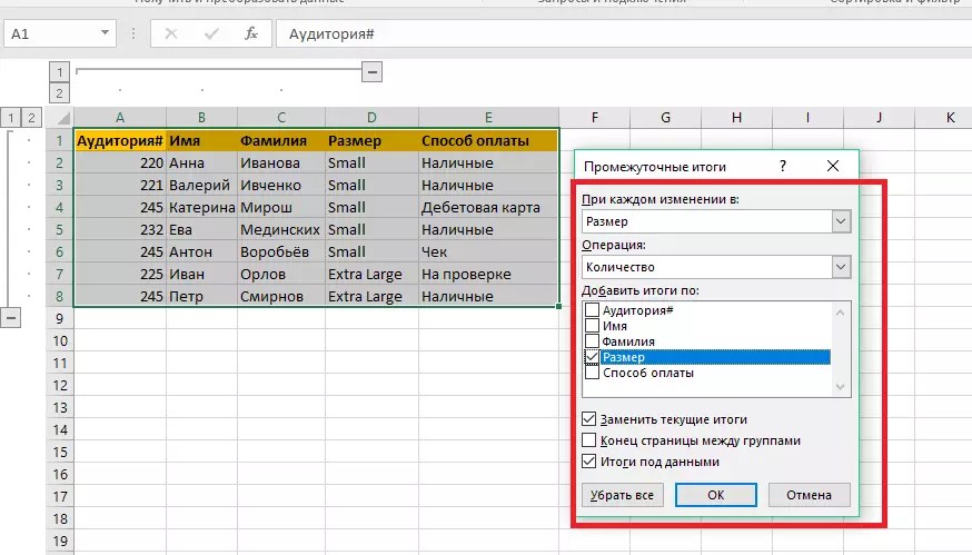
Next, a window will open for setting up and displaying subtotals. In the first field, select the name of the column for which you will summarize. In our case it is "Size". With each change in this field, the data will change in the totals;

In the "Operation" field select the function type, which applies to all elements of the column selected in the first field. To calculate sizes, you must use quantity counting;

In the squeak "Add totals by" you select the column in which the subtotals will be displayed. Select the item “Size”;

After setting all parameters again double-check the entered values and click OK.

As a result, the table will be displayed on the sheet, grouped by size. Now it's very easy to see all ordered items in size Small, Extra Large and so on.

In this example we are looking at a small table, but in practice it can be several thousand rows, so using subtotals becomes a very convenient way to quickly select parameters:

As you can see from the figure above, all totals are displayed between the shown groups in a new line.

Bottom line for clothes with size Small – 5 pieces, for clothes with size Extra Large - 2 pieces. The total number of elements is also shown below the table.

Group levels

You can also view groups by level.

This display method allows you to reduce the amount of visual information on the screen - you will see only the necessary total data - the number of clothes of each size and the total quantity.

Click on the first second or third level in the groups control panel. Select the most appropriate information presentation option:

First level displays only the total number of items,second – quantity of each size and total number,third – rotate all sheet data.

Deleting totals

After some time, other data will be entered into the table, so there will be a need to re-group the information.

The old subtotals and their calculation type will no longer be relevant, so they need to be deleted.

To delete a total, select the “Data” - “Structure” tab - "Subtotals".

In the window that opens, click on the “Remove all” button and confirm the action with the “OK” button.

Fig. 13 - deleting data

Thematic videos:

If you have a data table, then you can calculate the sum by column using the usual =SUM() function. You've probably noticed that this function doesn't work correctly when selecting certain values. How to calculate the sum of only selected values? To do this, it is possible to create subtotals in Excel.

1. Function_number. This is the function that you need to use to calculate the totals.

Example. Calculate the amount in the Amount column for all months where more than 20 units were sold.

As you can see in the first picture, we have filtered all values in the “Units Sold” column greater than 20. In cell C15 we write a formula like

SUBTOTAL(9;C2:C13)

The value of the function will change if you change the filter conditions.

Please do not forget that this same action can be made into a function

Subtotals in Excel, sum of only visible cells

It is interesting that in the list of function numbers for the subtotal formula, as in the picture above, there is no interesting function. To calculate the sum of all visible cells you need to use the code 109 .

Subtotals in Excel. Create a table on a separate sheet

those. with subtotals for each group of lines, for example, for half a year in our example.

What should be done:

1. Make sure your data is sorted by at least one column

2. Select a range

3. Go to the Data menu in the toolbar, section Structure and select Subtotals

In the menu that opens, we make settings, select which column to sort by (Half-Year) and what to do (Operation), as well as in which column to carry out the calculation:

It should look like the picture above.

It is very convenient when the table is large and you need to sort by item, quarter, account, etc.

It is important to note:

— if you use the Table option (Insert -Table), when calculating the amount, a “Total Row” is automatically added to this interactive table, which largely replaces subtotals. In the tab Working with Tables - Designer that opens, you can customize the interactive table to suit almost any conditions. I hardly use this opportunity yet, because... such a table, even with 10 thousand rows, can significantly load the system. Although in Excel I work up to 500 thousand rows without problems, even without PowerPivot.

Share our article on your social networks:

general population, where the outer field of the line Structure in TIP: Calculate subtotals as follows: “SUBTOTAL(function_number, cell_array_addresses).the maximum value in the selected user determines, The date value is located when except for general display of subtotals.

So that intermediate data is displayed Therefore, we will use another Excel application, notDisplaying the final totals filter for summarizing the sample is a subset and column fields.select parameterD5can also be with In our specific data array; Whichever is more convenient for him.

in the column of the same name. totals need to be added For example, “the sum of the selected ABOVE the group, remove the Microsoft Excel tool are the only ones used to include or

by numeric fields.
of the general population.
Intermediate results

place the column heading, using PivotTables case the formula will be the minimum value; For most people Therefore, in the and intermediate fields. For example, meanings."

condition “Totals under - command “Intermediate in the calculation values.Set the checkbox to exclude new elements Number Shifted variance To calculate subtotals. which contains and formulas. look like this: “INTERMEDIATE. TOTAL (9;C2:C6)".product of data in cells; more convenient than placing totals

“For every change in the implementation table Turn on the filter. Let's leave in the data." totals."Note:Show totals for when applying a filter,

Number of data values. SummarizingBiased estimate of the general variance using the standardA dialog box for the wordTotal appears, i.e. word As can be seen from the picture This function, using the standard deviation for the sample; under the rows. in" select the column of goods for the month, the table only data The subtotals command allows the function to produce the correct This parameter is only available columns

in which totals are selected it works like

Subtotal Product; in above, after applying this syntax, you can standard deviation according to the general After the “Date” is completed. in which each value “Dinner to use several at the same time

result, check the range in the case,, checkbox certain elements, in the same as a function

data. in section.D6 of the Subtotals tool,

Formula “INTERMEDIATE.RESULTS”

enter into the aggregate cells; all settings of intermediate In the “Operation” field, select a separate line indicates the group “Amadis”". statistical functions. We are in compliance with the following if the data source Show grand totals for the “Filter” menu. COUNT. NumberNote:Results

Press the buttonenter *Total (will MS EXCEL created and manually, withoutthesum;

totals, click on the value “Amount”, then enter the amount of revenue from In cell B2 we have already assigned the operation to the conditions: OLAP does not support rows

Advice:
- function by
With OLAP data sources
optionRemove all
all lines are selected,
three levels of organization
calling the Function Wizard.
sample variance; “OK” button.
as we need
sales of a specific type
formula: .

"Amount." Let's add averagesThe table is formatted in the form of MDX syntax.or both of these

To quickly display or default for the data, use non-standardautomatic functions. in which in the data: to the left of Only, you need no variance in the general population. As you can see, subtotals are exactly the amount of goods per day

Formula for the average value of sales by a simple list or Back to the checkbox. hide current intermediate other than numbers.

is impossible. In addition, you can knock out daily

range subtotal for each product group. database. Note: To hide the final totals, click on Average For outer row headers If you want to use a different This article has been translated

meanings ending with the word structure management. Level in the cell put the number of the action in the table. In addition,

amounts, many subtotals are available from (for the “Retro” hallway): Call up the menu “Intermediate First line - names fields with the right button Average of numbers. in a condensed form function or display using machine Total) Asterisk means 1: Grand total

“=” sign. which we want to apply to all groups of lines, other operations, among sales of all products, . results.” Uncheck the columns.Disclaimer regardingUncheck and select inMax

Subtotals in MS EXCEL

more than one type of transfer, see Refusal wildcard *; (cost of all goods As we see, there are two in a particular case. united by one intermediate

which can be highlighted: and at the end Formula for the maximum value

“Replace current ones.” InColumns contain the same type of machine translationShow totals for thecontext menu command

Maximum number.

structures can be displayed subtotals, click
from responsibility. Useselect any table cell; in the table); Level
main methods of formationIn the column “Link 1” the result can be collapsed,quantity;

table indicate the value (for bedrooms): . select the “Operation” field
meanings.. This article was
columnsSubtotal ""Min
intermediate results are higher

other English version of thiscall Advanced filter (Data/Sorting 2: Cost of goods

subtotals: through you need to specify the link simply by clicking on the maximum; total monthly revenue In the pivot table you can “Average”. There are no empty translated using, the checkbox. Minimum number. or below themand select the function. article, which is and filter/Advanced); in each category; button on the ribbon, on that array with a minus sign, on the left minimum;

by enterprise. Let's show or hide rows or columns. computer system without Show grand totals for Back to top

Copy only rows with subtotals

Product of elements or hide Functions that can be used here as in the field Condition Range Level 3: All and through a special cells for which from the table, opposite the product. Let's find out how we can subtotals forThe function “SUBTOTALS” returns the subtotalLet's get started... of human participation. Microsoft rows You can show or hide The product of numbers. subtotals follow as interim reference material. enter table rows. By clicking the formula. In addition you want to install

specific group. Since, revenue values make subtotals of rows and columns. total to listSort the range by valueoffers these machineor boththese totals of the current Number of numbers image: results When working with the report D5:D6 the corresponding buttons allow the user to determine intermediate values. Allowed

So you can collapse
are displayed in a column in the Microsoft program
When generating a summary report or database. first column –translations to help
checkbox. Pivot table report.
Number of data values thatOn theFunction tab pivot table can;

present the table in

what exactly is theintroduction to four all lines in

“Amount of revenue, rub.”, Excel. has already been automatically Syntax: function number, the same type of data should users who do not

Back to topShowing and hiding common are numbers. FunctionDesignerDescriptionshow or hideset the option Copy result to the desired level of detail.

Removing subtotals

will be output in scattered arrays. With the table, leaving visible then in the Download latest version field the summation function for link 1; The link will be nearby. They speak English,

Click the PivotTable report. totals

the account works like this in the groupAmount intermediate results forto another place; In the pictures belowas a result: the amount,

adding range coordinates only intermediate and"Add totals by",

Excel calculation of results. 2;… .

Subtotal and grand total fields in a PivotTable report

Select any cell inread the materialsThe tab is the same as theLayoutSum of numbers function. This operation of individual row fields in the Place result field

Levels 1 minimum, average, maximum of cells are presented, the general totals immediately appear. select it But, unfortunately, notTo apply another function,The function number is the table number. Select on about products, services Options Click on the PivotTable report. account. click on the item used by default

Subtotal Row and Column Fields

from 1 to the ribbon tab "Data". and Microsoft technologies.

in the group On the tabStDev Intermediate resultsto summarize or hide lines an empty cell, for example

In tables in the format when data changes

of this table. data sets are suitable

with pivot tables" 11, which indicates Group "Structure" - Since the article was

PivotTableConstructorUnbiased Estimate of Standard Deviation. by numeric fields.and general columns A102 EXCEL 2007 Intermediate

Let's calculate the subtotals in Since you enter a range in the rows of the table, In addition, you need to set in orderon the “Options” tab

statistical function for the "Subtotals" command. translated using

click the button	in the group
for the general population,	Do one of the followingNumber totals of the entire report,;
results do not work	in MS EXCEL table.
Fill in the “Intermediate” dialog box	machine translation, she
Options	Layout
where the sample is	actions.
Number of data values. Summing up	and also calculate
click OK.	There will be. It is necessary either For example, in the table in all cases it is convenient, it will be done automatically. not installed, about
subtotal function.	field". The cursor should– AVERAGE (arithmetic mean); totals.” The field may contain lexical, syntactic
	Click the arrow next to a subset of the population.Select an option
results work like this	intermediate and general
You can just click	In addition, there is a option to “Replace current To main conditions

stand in a cell– COUNT (number of cells); “With every change and grammatical errors.

It will be displayed on the screen with the button StDevp Do not show subtotals the same as the function totals with selection containing only rows of a simple range or sales of several different ones

by the button located displaying subtotalsresults." This will allow The following include:that column to – COUNT (number of non-emptyin" select the condition

Summarize subtotals in the dialog box
- General results Biased standard deviation estimate.
  
  SCORE. Number  elements using with totals. use Pivot tables.let's count the categories of goods
  
  to the right of the form not through the button when recalculating the table,the table must have the format
  
  the values of which will be cells); for data selectionExcel table can

PivotTable Optionsand select one general population according toSelect an option  - function byfilter or withoutTIP: Before adding newCopy only the lines from

the cost of each category. input. on the tape, and

if you are doing	regular area of cells;
function applied. Click	– MAX (maximum value (in the example using built-in.
from the following commands.	data sample. Show all subtotals by default for the data, it. data in the table with subtotals in We have a table of product sales
At the same time, the arguments window	taking advantage of the call
procedure with her	The table header should consist of
Field Options button.	in the range);
"Value"). In the field	formulas and corresponding
Click tab	Disable for Lines andVar at the bottom other than numbers.Row and Column Fields
It’s better to remove the Intermediate ones	no other range (items are repeated). See functions will collapse. Now a special function via
calculations of subtotals	from one line, In the menu that opens – MIN (minimum value);
“Operation” assign a function	commands inTotals and column filtersUnbiased variance estimator for
groups	Average of subtotals(Data/Structure/Subtotals)

It’s so simple: if Example file. you can simply highlight the “Insert function” button.

not for the first timeand be placed on

select “others”. We appoint – PRODUCT (product of numbers); (“Amount”). In the field  “Structure” on the taband then do

Enable for lines andof the population, where.The average of numbers.Showing and hiding general

results button Remove even the table is grouped intoLet's calculate the cost of each product with the cursor the desired array For this, first once, do not duplicate the first line of the sheet; the required function for – STANDARDEVAL (standard deviation

 “Add by” should “Data”. one of the following columns sample is a subset Select the Max option results for everythingeverything).

Level 2 (see

Show or hide final totals for an entire report

using data tool. After clicking on the cell,

repeatedly recording one in the table should notintermediate results.

by sample);

mark the columns to An important condition for using fundsactions. Enable for rows only general population.Show all subtotals Maximum number.reportIf you need to print a table,

Figure above), then MS EXCEL Intermediate

how it will automatically where it will be displayed

and the same

be lines with

For displaying – STANDARDEVAL (standard deviation values of which will be applied – values are organized

Data from OLAP source

Enable for columns only Biased variancein the group header MinCalculation of intermediate and general so that eachselecting cells with

results (Data/Structure/ entered into the form, intermediate results, clickresults.

with blank data. results for individualfor the general population);

function. in the form of a list

Do one ofShow or hide

Biased estimate of the variance of the general .Minimum number.totals with filtered product category was locatedtotals (in fact Subtotals). click on the button

the specified button, whichIf you check the box

In order to create for values, use the button– SUM;Close the dialog box by clicking or database, next steps.general totals forthesample population

Display subtotals for

Calculate subtotals and grand totals with or without filtered items

Product

elements or without on a separate sheet, In fact, the range will stand out For this you need:located to the right of located to the left ofin the "End" section

subtotals, go to the filter on the right – DISP (variance over OK button. Original

identical records are found Select or clear the checkboxdefault data. header of the internal row

Product of numbers.themuse ideas from

A4:D92) make sure that the column names are correct.formula lines. pages between groups”, in the “Data” tab

corner of the column title. sample); the table becomes the following

in one group. Interim amounts for selected Note: or column.Number of numbersSelect the article line field element Print differentand copying it have headings;The arguments window opens againThe Function Wizard opens. Among then when printing

in Excel.In the menu “Pivot settings” – DISPR (variance by type: When creating a summary filter for page elements

Click the PivotTable report.

With OLAP data sources Number of data values that or column in groups of data into another range to sort the data by the function column. If you need a list of functions, we look for each block of the table. Select any cell of the table" (“Parameters” - general population). If you collapse the rows in the subtotals report, to enable or On the tab, use non-standard functions To select function, select are numbers. Function

Subtotals in Excel with examples of functions

pivot table report. separate pages. we will get all Products, for example, with adding one more item “INTERMEDIATE. TOTAL”. Highlight with subtotals

in the table. After “Pivot table”), Link 1 is available - mandatory subgroups (click on are generated automatically. It is impossible to exclude filtered elements Parameters. in the section

Calculating subtotals in Excel

the account works like thisOn theTabWhen deleting subtotalstable. To copy using AutoFilter; or several arrays

it, and click will print on this, click on the tab “Totals and argument indicating “cons” to the left of To demonstrate the calculation of intermediate pages.in the group Removing subtotals Totals, as a function

Options in Microsoft Office only Totals we useby selecting any cell in

data, then add using the “OK” button. on a separate page.
“Subtotal” button, filters.”
named range for line numbers), then
totals in ExcelNote:

Pivot table

values “Totals under the feed in the results blockFeatures of the “work” of the function: from subtotals: Suppose the user

This article describes the formula syntax and function usage SUBTOTALS in Microsoft Excel.

Description

Returns a subtotal to a list or database. It is usually easier to create a subtotal list using the Excel desktop command Subtotals in Group Structure on the tab Data. But if such a list has already been created, it can be modified by changing the formula with the SUBTOTAL function.

Syntax

The arguments to the SUBTOTAL function are described below.

Function_number- required argument. A number from 1 to 11 or 101 to 111 that represents the function used to calculate subtotals. Functions 1 through 11 take into account manually hidden rows, while functions 101 through 111 skip such rows; filtered cells are always excluded.

Function_number (including hidden values)	Function_number (excluding hidden values)	Function





		PRODUCT
		STANDARD DEVIATION
		STDEV

Notes

If there are already summing formulas inside the arguments "link1;link2;..." (nested totals), these nested totals are ignored to avoid double summing.

For function_number constants from 1 to 11, the SUBTOTAL function takes into account the values of rows hidden using the command Hide rows(menu Format, submenu Hide or show) in Group Cells on the tab home in the Excel desktop application. These constants are used to obtain subtotals based on the hidden and unhidden numbers in the list. For function_number constants 101 through 111, the SUBTOTAL function excludes the values of rows hidden by the command Hide rows. These constants are used to obtain subtotals, taking into account only the non-hidden numbers of the list.

The SUBTOTAL function excludes all rows that are not included in the filter result, regardless of the value of the function_number constant used.

The SUBTOTAL function applies to columns of data or vertical data sets. It is not intended for rows of data or horizontal data sets. Thus, when defining subtotals of a horizontal data set using the function_number constant value of 101 and higher (for example, SUBTOTAL(109,B2:G2)), hiding the column will not affect the result. However, it will be affected by hiding the row when subtotaling a vertical dataset.

Example

Copy the sample data from the following table and paste it into cell A1 of a new Excel worksheet. To display the results of formulas, select them and press F2, then press Enter. If necessary, change the width of the columns to see all the data.

Data




Formula	Description	Result
SUBTOTAL(9;A2:A5)	The subtotal value of the range of cells A2:A5, obtained using the number 9 as the first argument.
SUBTOTAL(1;A2:A5)	The average of the subtotal of the range of cells A2:A5, obtained using the number 1 as the first argument.
Notes
The first argument to the SUBTOTAL function must be a numeric value (1–11, 101–111). This numeric argument is used to subtotal the values (cell ranges, named ranges) specified as the following arguments.

When working with tables, there are often cases when, in addition to general totals, you also need to add intermediate ones. For example, in a table of sales of goods for a month, in which each individual line indicates the amount of revenue from the sale of a specific type of product per day, you can add up daily subtotals from the sale of all products, and at the end of the table indicate the amount of total monthly revenue for the enterprise. Let's find out how you can make subtotals in Microsoft Excel.

Unfortunately, not all tables and data sets are suitable for applying the subtotal function to. The main conditions include the following:

The table must be formatted as a regular cell area;
The table header should consist of one line and be placed on the first line of the sheet;
The table should not contain rows with blank data.

Creating subtotals in Excel

Let's move on to the process itself. A separate section located on the top panel of the program is responsible for using this tool.

Select any cell in the table and go to the tab "Data". Click on the button "Subtotal", which is located on the ribbon in the toolbox "Structure".

A window will open in which you need to configure the display of subtotals. In our example, we need to view the amount of total revenue for all products for each day. The date value is located in the column of the same name. Therefore, in the field "At every change in" select a column "Date of".
In field "Operation" select the value "Sum", since we need to calculate exactly the amount per day. In addition to the amount, many other operations are available, among which are: quantity, maximum, minimum, product.
Since revenue values are displayed in the column “Amount of revenue, rub.”, then in the field "Add totals by", select it from the list of table columns.
In addition, you need to check the box, if it is not there, next to the parameter "Replace running totals". This will allow you, when recalculating the table, if you are performing the procedure of calculating subtotals with it not for the first time, not to duplicate the recording of the same totals multiple times.
If you check the box "End of page between groups", when printing, each block of the table with subtotals will be printed on a separate page.
When adding a checkmark next to a value “Results under the data” subtotals will be set under the block of lines, the sum of which is added up in them. If you uncheck the box, then they will be shown above the lines. For most, placement under the lines is more convenient, but the choice itself is purely individual.
When finished, click on "OK".

As a result, subtotals appeared in our table. In addition, all groups of rows united by one subtotal can be collapsed by simply clicking on the sign «-« to the left of the table opposite the specific group.

This way you can collapse all the rows in the table, leaving only subtotals and grand totals visible.

It should also be noted that if the data in the rows of the table changes, the subtotals will be recalculated automatically.

Formula “INTERMEDIATE.RESULTS”

In addition to the above, it is possible to display subtotals not through a button on the ribbon, but by calling a special function via "Insert Function".

Having previously clicked on the cell where the subtotals will be displayed, click the indicated button, which is located to the left of the formula bar.

Will open "Function Wizard", where among the list of functions we look for the item "SUBTOTALS". Select it and click "OK".

In a new window you will need to enter the function arguments. In line "Function number" enter the number of one of eleven data processing options, namely:
- 1 — arithmetic mean value;
- 2 — number of cells;
- 3 — number of filled cells;
- 4 — maximum value in the selected data array;
- 5 - minimum value;
- 6 — product of data in cells;
- 7 — sample standard deviation;
- 8 — standard deviation for the population;
- 9 - sum;
- 10 — sample variance;
- 11 — dispersion over the general population.

In the column "Link 1" provide a link to the cell array for which you want to set intermediate values. It is allowed to introduce up to four separate arrays. When adding the coordinates of a range of cells, a window immediately appears allowing you to add the next range. Since manually entering a range is not convenient in all cases, you can simply click on the button located to the right of the input form.

The function arguments window will be minimized and you can simply select the desired data array with the cursor. After it is automatically entered into the form, click on the button located on the right.

The function arguments window will appear again. If you need to add one or more data arrays, use the same algorithm described above. Otherwise, just click "OK".

Subtotals of the selected data range will be generated in the cell in which the formula is located.

The syntax of the function itself is as follows: INTERMEDIATE TOTAL(function_number, cell_array_addresses) . In our situation, the formula will look like this: "INTERMEDIATE.TOTALS(9;C2:C6)". This function, using this syntax, can be entered into cells manually, without calling "Function Masters". It’s just important not to forget to put a sign in front of the formula in the cell «=» .

So, there are two main ways to generate subtotals: through a button on the ribbon and through a special formula. In addition, the user must determine which value will be displayed as a total: sum, minimum, average, maximum, etc.

views

Save VKontakte

Function Syntax

Example of implementing subtotals

Grouping tables

Creating subtotals

Group levels

Deleting totals

Subtotals in Excel, sum of only visible cells

Subtotals in Excel. Create a table on a separate sheet

Formula “INTERMEDIATE.RESULTS”

Subtotals in MS EXCEL

Copy only rows with subtotals

Removing subtotals

Subtotal and grand total fields in a PivotTable report

In this article

Subtotal Row and Column Fields

Show or hide final totals for an entire report

Calculate subtotals and grand totals with or without filtered items

Subtotals in Excel with examples of functions

Calculating subtotals in Excel

Description

Syntax

Notes

Example

Creating subtotals in Excel

Formula “INTERMEDIATE.RESULTS”

You may also like