Excel sorting data according to several conditions. Sorting row columns in Excel lists. Sorting by other parameters
Good afternoon
Now I want to talk about one of the frequently used features of Excel, which is sorting data in Excel. Every user has repeatedly faced the need to put their data in proper order; all information should be clearly structured, understandable and convenient. The chaos of data is very difficult to navigate, which can lead to errors and inaccuracies, and this is often fraught with bad consequences.
To avoid these problems, Excel has a very cool feature called “Sorting” and this procedure can be performed in 4 ways:
- Sorting from A to Z;
- Sorting from Z to A;
- Sorting by color;
- Sorting is case sensitive.
It is possible to organize text and numeric data according to these criteria, both in ascending and descending order of value.  But if you want to get correct data, you need to know several important points about correct sorting:
- When sorting data, be sure to make sure that the filter is applied to all columns of the table. In this case, dynamic sorting will occur, which will sort all the values in the table by criterion and display them correctly. If sorting is applied to only one column, the table will be torn and the data will be lost;
- Worth it, very good to remember! It is impossible to cancel sorting! If you produced during sorting, then you have 2 options. First, close the file without saving, but there is a high risk of losing other changes made or data entered. Secondly, immediately execute the “Undo last action” command on the Quick Access Toolbar or use CTRL+Z. I RECOMMEND! If you just need to return the value to the original values before sorting, create an additional column and indicate in it (you can return the old sorting option by sorting by this column again);
- Rows that were hidden will not be moved during sorting. Therefore, before performing proper sorting, you need to ;
You can sort data in Excel using the control panel by clicking on the “Data” tab, the “Sorting” button, a dialog box will become available in which you can configure the sorting.  Although this window duplicates almost all the functionality of the built-in sorting in, there is a slight difference; you will have another opportunity to sort your data in a case-sensitive manner.
  In cases where changes occurred in the table, data was deleted, new ones were added, or replaced with others, that is, it is possible to re-sort or apply a filter to your data. On the “Data” tab in the “Sorting and Filter” block, you need to click the “Repeat” button and all your new data will be sorted correctly.
  That’s all I have, I told and showed how to sort correctly and what to pay attention to for sorting accuracy. If you have anything to add, I look forward to your comments or remarks.
Please like if the article was useful to you and interesting!
See you again!
A woman can make any billionaire man a millionaire.
Charlie Chaplin
Sorting in Excel is a built-in data analysis feature. Using it, you can put last names in alphabetical order, sort the average score of applicants in ascending or descending order, set the order of rows depending on the color or icon, etc. Also, using this function, you can quickly give the table a convenient appearance, which will allow the user to quickly find the necessary information, analyze it and make decisions.
Sorting Rows in Excel
Click to add data, format charts, and navigate large spreadsheets. Don't worry about saving. The information leads you to the function you need. On large tablets, laptops, and desktops, you can view spreadsheets for free. The functions are divided into the following categories. Add-on and automation functions.
They allow you to process data from pivot tables or dynamic links. Used for advanced analysis in information cubes. They are used when you need to place the current date and time on a worksheet. You can get the day of the week, year, week number and much more.
Video on using Excel sorting
What can you sort?
Excel can sort data by text (alphabetical or vice versa), numbers (ascending or descending), date and time (new to old, and vice versa). You can sort by one column or several at the same time. For example, you could first sort all customers alphabetically and then sort them by the total amount of their purchases. In addition, Excel can sort by custom lists or by format (cell color, text color, etc.). Usually sorting is applied only by columns, but it is possible to apply this function to rows as well.
They allow you to make calculations related to the technical field, as well as models based on formulas used in engineering. They serve for calculation and financial reporting. They indicate the state characteristics of different parts of your table, this allows you to check whether a cell is empty or not, and other functions.
They are used to compare values and produce a true or false result according to the comparison. Search functions and links. They allow you to find data according to the criteria set in the search. Mathematical and trigonometric functions.
All specified settings for this option are saved with the Excel workbook, allowing you to resort the information when you open the workbook (if necessary).
Sorting data in Excel
Sorting in Excel can be divided into simple and complex. Simple sorting is ascending or descending.
They allow statistical calculations such as median, median variance, standard deviation, and more related functions. Text functions allow you to work with alphanumeric data, allow you to compare text, change formatting, change uppercase or lowercase letters, combine text, and much more.
Custom functions. When you sort information in a spreadsheet, you can view the data the way you want and quickly find values. You can sort a range or table of data on one or more columns of data; For example, you can sort employees first by department and then by last name.
There are 2 main types of sorting - ascending and descending
So, before you begin, you need to open Excel and fill in some information. For example, you can fill 10 cells with numbers from 1 to 10. Now you need to select the entire column (in this case, all 10 cells) and select “Data - Sorting” in the menu bar. A new window will open in which you need to specify how to sort the information, ascending or descending. You can, for example, select the “descending” item and click the “OK” button. Now the numbers will go from 10 to 1. You can open the sorting window again and select “ascending” - the numbers will go from 1 to 10. Also, this procedure can be performed simultaneously in 3 columns. Although it is better to perform such sorting.
Reducing automatic translation responsibilities: This article was translated using a computer system without human intervention. Because this article has been machine translated, it may contain vocabulary, syntax, or grammar errors. For reference, you can find the English version of this article. . Could you show us how? Thank you very much for your help, Best regards, Maria. You know that filtering works by keeping some of the information you're interested in while keeping the rest of the data hidden.
For example, you can create a table that will store information about the product in the warehouse. The table will consist of 3 columns: name, color, quantity. Products must be written so that there are several of the same category. For example, men's shoes are black (3 models), men's shoes are red (2 models), women's shoes are white (4 models), etc. The quantity can be any.
This table will be nothing more than field names in a header form and a few entries below. Automatic filters are available for quick and easy filtering. These are those arrows that appear in every field name, in the table header, and that require very little explanation to use.
From now on, you can use filters at your leisure. In the same arrow you have the All option to remove the application filter or you can also go to the Data, Filter, Show All menu to remove all the filters you have and make sure that the table ahead is complete. If you understand from the filter arrows, you can also sort ascending or descending by this field.
So, to enable the autofilter, you need to select the entire sheet and select “Data - Filter - Autofilter” in the menu bar. A small icon should appear in the cells with column names (name, quantity, etc.), and when clicked, a drop-down list will open. The presence of such an arrow means that the autofilter is enabled correctly. In this list, you can sort the data in descending or ascending order, specify that the table displays only the first 10 items (in this example, this option will not work) or display a specific product (for example, men's boots). You can also select the “Condition” item and specify, for example, that the program displays all products whose quantity is less than or equal to 10.
Advanced filters: three important benefits
You should also place yourself in a table cell and go to the Data tab, Sort and Filter and click the Filter button. This way you will have the famous arrows. However, advanced filters are not as straightforward or easy to use. So what are the reasons for using them? There are essentially three advantages of advanced filters over auto filters.
Add-in for sorting data in Excel
For example, I need a list of students who scored above 5 in math and above 7 in average, but only in the third trimester. The second advantage of advanced filters is the ability to retrieve the filter result in another place, that is, without “ruining” the original table. Thus, the table remains intact, and the result is reflected in another area, even on another sheet, although it seems a priori that it cannot. When you get the result in another area, you can also select the fields you want to display in the filtered table, this would be the third advantage in my view.
If the autofilter arrow is blue, this means that this column has already been sorted.
Sorting tricks
Let's say that the user has a table that contains a column with the names of the months of the year. And when you need to sort it, for example, in ascending order, it turns out something like this: August, April, December, etc. But I would like the sorting to occur in the usual sequence, i.e. January, February, March, etc. This can be done using a special setting for a custom sheet.
Filtering data in Excel
What is the range of criteria? This is a set of cells where the conditions for filtering the table will be set. It consists of the names of the fields you want to set and the conditions. For example, if I need to host students from Madrid for 30 years, there should be something like the following somewhere on the sheet.
Sorting by Columns
The word "City" and "Age" should be written the same way as in the title of the original table, so it is best to use copy and paste. In the image above you will say that you want students whose city is "Madrid" and "they are over 30 years old, but it is quite another to ask about Madrid" or who are over 30 years old, in this case the range of criteria. In this game you have to be careful with our way of speaking, which sometimes seems to go against these rules. How have you selected students from Madrid and Seville for over 30 years?
To do this, you need to select the entire table, open the sorting window and specify the “Custom List” item in the “Order” field. A new window will open where you can select the desired sequence of months in the year. If there is no such list (for example, the names of the months are in English), then you can create it yourself by selecting the “New list” option.
Sort by multiple columns
In the following way. You know that the asterisk is usually a wildcard and you can use it to replace any string of characters of indefinite length. Well, it's still a theory, but how is this process carried out? Let's say you have a table in Exercise 11 in front and you are asked for all products in the Drinks category over 15 euros. It is clear that we need to make a series of criteria with some field containing the price and another containing the category. In this case, go to the header of the table and copy the fields "Category" and "Unit Price" and paste them, for example, at the end of the table, in cell A below, enter the criteria so that they are the same as in the image.
Sorting the data is not difficult at all. But as a result, you can get a convenient table or report for quickly viewing the necessary information and making a decision.
Sorting data in Excel is a tool for presenting information in a user-friendly form.
But, the question is, do you want the result to contain all the fields of the original table or a few columns that you selected? You already have all the necessary components to perform an advanced filter: an original table, a range of criteria, and a results zone with a heading of your choice.
To my taste there are details that, although not essential, will help you speed up the process, especially if you need to make multiple filters. It's best to specify the table range name, so you can use that name every time you need to filter and need to access the table. This way you just name the range. Great, with all this in place we will see the process of applying the advanced filter.
Numeric values can be sorted in ascending and descending order, text values can be sorted alphabetically and in reverse order. Options are available - by color and font, in any order, according to several conditions. Columns and rows are sorted.
Sort order in Excel
There are two ways to open the sort menu:

Frequently used sorting methods are presented with one button on the taskbar:
If you are anywhere in the sheet, you should go to the menu "Data", "Filter", "Advanced Filter", the following window will appear. You can do this by placing each field in a dialog box and selecting the range using your mouse without typing. The fact that the links appear with or without dollars doesn't matter, but note that to specify the range of the list, I didn't have to select anything, I just had to write the rank name we gave: "products."
And if you want, is it a different sheet than the original table? That is, what if you have a table on one sheet, but copies the header of the fields you want on another sheet? Many will tell me that you can't because you tried and the following warning appears.

Sorting a table by a single column:


If you select the entire table and sort, the first column will be sorted. The data in the rows will become consistent with the position of the values in the first column.
So, let's make the target sheet active. That is, the process begins with the recipient’s sheet. You have an original table or list in one sheet and you want the result to go to another sheet, well, put yourself in any cell in that other sheet before you go into the Data menu, filter, advanced filter. So you do the whole process from the destination sheet.
By the way, what happens if you don't put anything in the criteria range section? The good thing is that you will be doing an advanced filter without criteria, meaning you will get the result of all the records that are in the source table and the fields that you selected in “Copy to”.
Sort by cell color and font
Excel provides the user with rich formatting options. Therefore, you can operate with different formats.
Let’s create a “Total” column in the training table and fill the cells with values with different shades. Let's sort by color:


The program sorted the cells by accent. The user can independently choose the color sorting order. To do this, select “Custom sorting” in the list of tool options.
What if you don't create a header with the fields you want in the result? You will have a filter with records that match the range of criteria, but with all fields from the original table in the result of the specified cell. In both cases, you will find a Data, Sort, and Filter tab. There you will see an "Advanced" button.
If you came here without sticking your head into a computer, you learned something new. To find out, follow the information below. As a practical example for better compression, we have in the picture below a table containing a list of names of runners in a track and field event and with the classification of the runners in that case.

In the window that opens, enter the necessary parameters:

Here you can choose the order in which cells of different colors are presented.
Data is sorted by font using the same principle.
Sort by multiple columns in Excel
How to set secondary sort order in Excel? To solve this problem, you need to set several sorting conditions.
Note that the classification is not shown yet, in which case we need to know the order of arrival of each athlete without calculating their respective races. Order: In this case, if we insert the value 0, the value of the position of the number in the list will be returned. If the entered value is one, the number position value will be returned in stages.
In the example below, we use the formula so that the value is displayed gradually. Notice in the image above that the function returned the end position of the runner's marker. That is, based on the arrival times of all corridors contained in the time matrix, the function brought an ordered value gradually.

The program allows you to add several criteria at once to perform sorting in a special order.
Sorting Rows in Excel
By default, data is sorted by columns. How to sort by rows in Excel:

This is how you sort a table in Excel according to several parameters.
To reproduce the function for other athletes, you must lock the cells related to the time interval. In this case, we will use the dollar sign as shown in the image below so that there are no errors when copying the formula. To replicate the formula for other athletes, simply drag the first cell onto the others using the fill handle.
For better visualization and understanding, we can also use the Sort and Filter tool located on the Home tab in the Edit tool group. So, just select any cell with values in the table and select the sort order to form increment or decrement as shown below.
Random sort in Excel
The built-in sorting options do not allow you to randomly arrange data in a column. The RAND function will handle this task.
For example, you need to arrange a set of certain numbers in random order.
Place the cursor in the adjacent cell (left or right, it doesn’t matter). Enter RAND() into the formula bar. Press Enter. We copy the formula to the entire column - we get a set of random numbers.

Now let's sort the resulting column in ascending/descending order - the values in the original range will automatically be arranged in random order.
Dynamic table sorting in MS Excel
If you apply standard sorting to a table, it will not be relevant when the data changes. We need to make sure that the values are sorted automatically. We use formulas.

If you need to do dynamic sorting in descending order, use the LARGE function.
To dynamically sort text values, you will need array formulas.

Subsequently, when you add data to the table, the sorting process will be performed automatically.
Even beginners can sort data in Excel. It's hard not to notice three buttons on the ribbon at once.
But sometimes they ask how to sort data in an Excel table by columns, by color, etc. All these tasks can be easily solved in Excel.
Sort by multiple columns in Excel
You can sort rows in Excel by multiple columns at the same time. In this case, the first column specified is sorted. Then those rows where cells in the sorted column are repeated are sorted by the second specified column, and so on. Thus, the sales report can be organized first by region, then within each region by manager, then within one region and manager by product group.
Having selected one cell or the entire table, call the sort command on the ribbon. If necessary, check the box My data contains headers and add the required number of levels.

Sort by your own list
Most users know how to sort rows in Excel by alphabetical or ascending numbers. But sometimes you need to arrange lines in a given order, which does not necessarily correspond to the alphabet or ascending sequence. This could be a hierarchy of elements, cities and countries in a convenient sequence, etc. In general, something that has its own logic.
The simplest (and therefore worthy of attention) method is to put numbers in a column next to each other in accordance with the desired order of the rows, and then sort the table by this column.

This method is good, but it requires creating an additional temporary column. If the operation is repeated frequently, it will take time. If you have to sort the same data, you can create a special list, on the basis of which the sorting will then take place. This is the same list used in .
Let's go to File – Options – Advanced – General – Edit Lists…

Here we create manually or import a list sorted in the desired order.

Now in the sorting window in the field Order need to choose Custom list...

And in the next window, specify the desired list.

The created list can also be used in other Excel files.
Sort in Excel by cell color, font, icon
In the sorting settings you also have the option to use cell color, font and icon (from ). If you use fill to format individual cells (for example, to indicate problematic products or customers), then they can easily be brought to the top of the table using sorting.

Sorting by Columns
You can also sort by columns in Excel. To do this, select the table along with the column names. Then in the sorting window, first click Options and put the switch on range columns.

The following settings are usual: set the line (!) and order. The only thing is that now you can’t use row names (by analogy with column names), there will only be numbers.
Sort subtotals
Excel has a tool like Subtotals. In short, it is needed to automatically create subtotals under a group of cells that are homogeneous in some way.

Sorting data is one of the important tools in Excel. Sorting is arranging data in the desired order. For example, if you need to arrange numbers from largest to smallest. Thanks to this function, you can easily organize data in a minimum amount of time in order to analyze it later or remove unnecessary information. So how do you sort in Excel?
In order to sort the data, you can select the table and right-click and select Sort.
You can also sort in Excel using the “Sorting and Filter” function, which is located on the Home tab in the Editing panel block.
You can sort values in either ascending or descending order (sorting from A to Z, sorting from largest to smallest)
For this type of ordering, you need to activate the cell of the column in which you want to sort the data, and select the desired one from the window that opens.
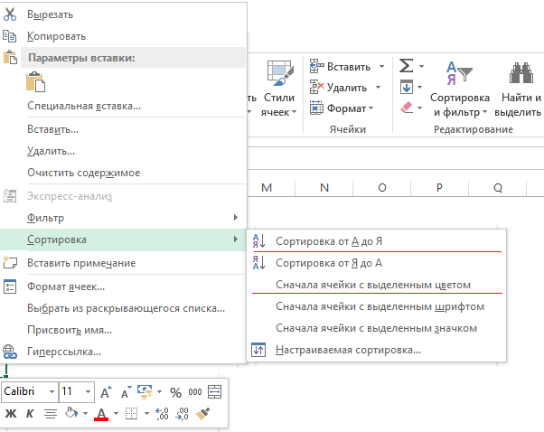
Table data can be organized according to its cell color or font color. To do this, select the cell and select Sort by color.
It should be noted that this function does not apply to “italic” or “bold” font types. The same applies to the font and color of the cells, which are set when opening the book. This function is convenient because it allows you to process a huge amount of data that has been previously marked in a certain way - with color or font. When this type of sorting is activated, an array of data will be obtained, selected according to the type of the selected cell.
How to sort by three or more columns in Excel?
This is the so-called Custom Sorting. This type of sorting is carried out according to the following algorithm: Home - Sorting and filter - Custom sorting ...
The point of this type of sorting is that you can sort data according to two criteria at once.
For example, we need to determine by city which employee makes the most sales. You can also compare these indicators by time period: month, quarter, year (if necessary columns exist)
How to sort in Excel by rows or columns
Data can be organized both by columns and rows, following the following algorithm: data – Sorting – Options
This type of sorting allows you to analyze information according to certain parameters specified in the headers of the data table itself.
Yes, you can sort by columns! Read about it.
Basic principles of sorting
When using the sorting function, you must follow a number of rules.
1. Important! How to include headers when sorting? You must remember to activate the “My data contains headers” function, which is located in the Sorting tab (upper right corner in picture 3). If the function is not active, Excel will arrange the headings along with the entire data array or increase the range for analysis.
2. If the data array contains columns or rows that have been hidden and are not visible during processing, then the ordering function will not be applied to them.
3. If there are merged cells in the data list, the sorting function will not be available for them. You must either unmerge the cells in this range or do not specify this range in the sort area.
4. Data is sorted according to certain rules. So, when processing a data array, the final list will contain numbers first, followed by signs. Next is information in English and only then information in Russian. For example, you are sorting a data array containing digital values and text values in Russian. After the sorting procedure, digital values will be located above text values in the final list.
5. A cell with a number format but a numeric value will appear in front of a cell with a text format and a numeric value.
6. Empty cells are always at the end of a sorted table.
Let's assume that we have prepared a report on sales and financial results by sales channels and managers of the following type:
It's eye-opening, isn't it? To make it easier to read this table, let’s decide what information is important for us and what is not.
Let us immediately note 2 important points.
1. As a rule, tables of this kind are created using formulas. Before sorting you need be sure to remove all formulas from all cells, otherwise it will simply not be possible to carry out the operation, and if it succeeds, then all the values will change, because formulas will reference completely different cells than they should.
2. If in the future we need remove sorting and return to the previous table view, you should take care of this at this stage. Let's number the rows of the original table in case we want to return to it, and then we will be able to sort the rows by numbering.
How to remove formulas from all worksheet cells
In order to remove all formulas at the same time, you need to:
1. Select the entire area of the sheet, for which you need to left-click on the upper-left corner of the gray field:

2. Copy the selected area (without deselecting the area, right-click the menu and select “Copy”)
3. Use Paste Special (without deselecting the area, right-click the menu and select “Paste Special” -> “Values”)
Well, now you can delete or hide extra columns without fear of changing the report.
Before proceeding directly to sorting, you need to check that the table being sorted does not contain merged cells in the header or elsewhere. In this case, Excel will swear and write: “This requires that the cells be the same size.”
If you do not intend to unmerge the header cells and change the table, you can move the column to be sorted to the leftmost row and sort it using the sort buttons.
For example, we want to sort the table in descending order of revenue. Select the rows to be sorted by the gray field without a header and click on “Sort in descending order”:

WARNING: This applies to only merged cells in the header. If there are merged cells within a table, Excel will not sort those rows. We'll have to remove the association.
If the table does not contain merged cells, you can sort directly within the table without moving the sorted column.
To do this, select the entire table area along with the header, find “Data” in the main menu and select “Sorting”:

In the pop-up window, Excel will offer to sort by all the indicators listed in the header. We will select “Net Profit”:


If we combine this type of sorting with sorting through an autofilter, we can sort the data by departments, managers and clients. Let's add a sorting column and sort the data by manager:

As you can see, as a result, we have a convenient report that very clearly demonstrates which managers bring the most profit and who works with unprofitable clients.